 Colliers Insights Team
One of the most important (and perplexing) concepts we run into on a daily basis in the GSA property marketplace is the concept of “cap rate.” The cap rate has long been used as a benchmark for pricing commercial real estate across all product types but in the 1990s and into the 2000s became more widely applied as the primary tool for property valuation — as real estate emerged as a mainstream asset class due to the flood of capital into the sector.
Plus: GSA occupancy of new buildings has dwindled | New measures for downsizing federal real estate
The concept of the cap rate, short for capitalization rate, comes from bond pricing, specifically annuity bond pricing, where the annual income from the bond is constant and extends into perpetuity — as expressed in the formula:
Capitalization rate = annual Income / value
or conversely:
Value = annual income / capitalization rate
The important concept here is the term “perpetuity” and the notion that the annual income derived from the asset being valued will continue on forever. Using the cap rate makes sense when applied to multitenant office, industrial, retail and multifamily product because annual or periodic rent escalations within the leases that generate the revenue for these assets, along with overall market inflation, create an environment where net operating income (NOI) is projected to remain stable or increase over time. This is also the case with single-tenant, triple net, long-term leased product where rent escalates and operating expenses are primarily the responsibility of the tenant, making NOI more predictable. In all of the above cases, because of this predictability and upward trend, residual values at the end of the investor’s holding period are much more stable and predictable.
Plus: How the Murrah Building bombing changed federal security | How open-plan office spaces can fail
However, within the GSA-leased property marketplace, the variance in GSA lease structures — and resulting annual rent obligation structures within these leases — does not always provide a stream of annual NOIs that are increasing or even remaining stable over time. Therefore, the cap rate for a GSA-leased property is meaningless unless it is placed in context.
As a result, a number of different methods have emerged in calculating cap rates for GSA-leased properties. The correctness or incorrectness — or accuracy or inaccuracy — of these various methods then comes down to a matter of individual preference. The problem arises when cap rates among various GSA-leased property transactions are compared, but the methods used to calculate those cap rates are different – or the context or circumstances present within each individual data point vary.
Let’s look at the example of the long-term, GSA-leased asset where the annual rent obligation is flat over time and the expense recoveries are deemed to be sufficient to cover future expense inflation, providing a level NOI over the full-lease term. In this instance, dividing the projected Year 1 NOI into the sale price to determine the cap rate, or dividing the NOI by the cap rate to determine value, makes sense.
However, because the vast majority of GSA leases contain soft terms (where the GSA has the right to terminate), the annual rent obligation structure will frequently decrease at some point during the lease term. In the case of a newly commencing GSA lease with a term of 10 years with five years firm (non-cancellable), where the shell and operating expense component of rent is flat through the entire lease and tenant improvement costs are amortized only over the first five years of firm term, there is a decrease in the rent obligation in Year 6 — and therefore a projected decrease in NOI during the last five years of the lease. A simple example is illustrated below (ignoring inflation/CPI escalation):
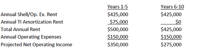
For illustrative purposes, if we assume this asset is priced at $3,500,000, based on a determination of the cap rate using the formula Year 1 NOI / Value, the cap rate is 10 percent. However, the yield drops in Year 6 to 7.86 percent.
In this case, neither 10 percent nor 7.86 percent accurately represent the cap rate of this asset, as the initial yield of 10 percent is not maintained during Years 6 to 10 of the lease, and the projected yield starting in Year 6 of 7.86 percent does not take into account the additional rental income received during the first five years of the lease. As a result, how does the investor convert this uneven cash flow to a cap rate that can be compared to other GSA-leased asset sales? Two methods provide possible solutions to this problem.
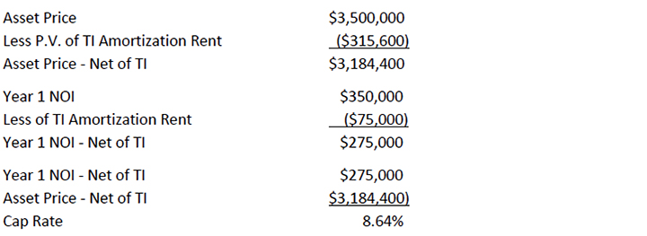
The first method separates the component of the pricing of the asset that is attributable to the TI Amortization Rent so that the cap rate can be determined on the remaining NOI — the portion of the NOI that is maintained during the full term of the lease. In the example above, Annual TI Amortization Rent of $75,000, paid monthly over a 5-year period, using 7 percent as the annual discount rate, has a present value of approximately $315,600. The cap rate is then calculated as follows:
The second and simpler method calculates the average projected yield over the lease term. Again using the above example, with a projected yield in Years 1 to 5 of 10 percent, and 7.86 percent in Years 6 to 10, the average yield over the full 10-year term is 8.93 percent. This can also be calculated by taking the average projected NOI over the lease term of $312,500, divided by the asset price of $3,500,000.
In certain cases, although occurring much less frequently, there are GSA leases in which the annual rent obligation increases during the lease term, even though the TI component “de-amortizes” after the firm term of the lease. An example is illustrated below (ignoring inflation/CPI escalation):
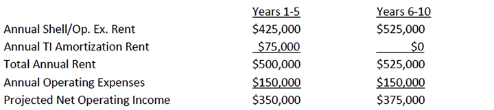
For illustrative purposes, if we assume this asset is priced at $4,250,000, based on a determination of the cap rate using the formula Year 1 NOI / Value, the cap rate is 8.24 percent. However, the yield increases in Year 6 to 8.82 percent. In this case, it would be perfectly acceptable to use 8.24 percent as the cap rate for this asset. However, this does not take into account the increased yield beginning in Year 6 and the fact that an investor may accept a lower initial yield in anticipation of a future increase — as compared to the initial yield for a 10-year lease term that is flat for the full lease term. The alternative again is to calculate the average yield over the full lease term. With a projected yield of 8.24 percent for Years 1 to 5 and 8.82 percent for Years 6 to 10, the average yield over the full lease term is 8.53 percent.
When we look at all of the examples above, it is easy to see how challenging it can be to compare published cap rates across the full spectrum of GSA-leased asset sales in determining a “market cap rate” for a particular GSA-leased asset being evaluated, by looking only at remaining lease term in addition to other factors such as location, agency and deal size. With the vast array of lease and rent structures across the GSA lease inventory, it is important for each investor to determine the cap rate methodology that is the most relevant to the particular investment requirements.
Bob is Senior Vice President of Colliers International in Atlanta and a member of the firm’s Government Solutions practice group, a comprehensive services platform focused solely on government real estate. Bob and his partner Darrin Kennedy in Los Angeles form Colliers GSAXCHANGE, the investment sales arm of Colliers Government Solutions.

 Workplace Advisory